Graph Representations
Graph data structure is represented using following representations
- Adjacency Matrix
- Adjacency List
- Adjacency Multilists
- Weighted Edges
1. Adjacency Matrix
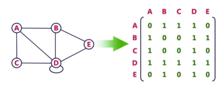
In this representation, graph can be represented using a matrix of size total number of vertices by total number of vertices; means if a graph with 4 vertices can be represented using a matrix of 4X4 size.
In this matrix, rows and columns both represent vertices.
This matrix is filled with either 1 or 0. Here, 1 represents there is an edge from row vertex to column vertex and 0 represents there is no edge from row vertex to column vertex.
Structure
- For unweighted graphs:
matrix[i][j] = 1if there is an edge fromitoj, else0.
- For weighted graphs:
matrix[i][j] = weightif there is an edge fromitoj, else0or∞.
Example

Time & Space:
- Space:
O(V^2) - Add edge:
O(1) - Check edge existence:
O(1) - Iterate over neighbors:
O(V)
Advantages of Adjacency Matrix
- Easy to implement
- Quick edge lookup
Disadvantages of Adjacency Matrix
- Wastes space for sparse graphs
- Inefficient for large graphs with few edges
2. Adjacency List
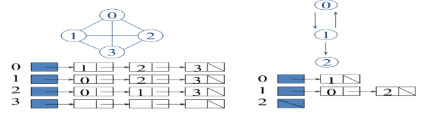
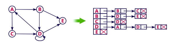
An adjacency list represents a graph as an array of lists. The index of the array represents a vertex, and the list at that index contains the neighbors of that vertex.
Structure
- For unweighted graphs: each list contains adjacent vertices.
- For weighted graphs: each list contains
(neighbor, weight)pairs.
Example
So that we can access the adjacency list for any vertex in O(1) time.
Another type of representation is given below.
Example: consider the following directed graph representation implemented using linked list.
This representation can also be implemented using array

Time & Space
- Space:
O(V + E) - Add edge:
O(1) - Check edge existence:
O(degree(v)) - Iterate over neighbors:
O(degree(v))
Advantages of Adjacency List
- Space-efficient for sparse graphs
- Efficient to traverse neighbors
Disadvantages of Adjacency List
- Slower to check if an edge exists
- Less suitable for dense graphs
3. Edge List
An Edge List is the simplest graph representation, where a graph is represented as a list of its edges. Each edge is stored as a pair (or triplet) of vertices, and optionally a weight if the graph is weighted.
In this representation, the graph is viewed primarily as a collection of edges, with no direct access to neighbor vertices of a given node unless we search the list.
This structure is often used in graph algorithms that work directly with edges, such as Kruskal’s Minimum Spanning Tree algorithm.
Structure of an Edge List Node
Each edge entry in the list contains:
vertex1: one endpointvertex2: the other endpoint(optional) weight: if the graph is weighted
All edges are stored in a flat list or array, one per entry.
For an undirected graph:
- Each edge is stored only once as
(u, v)or(u, v, weight).
For a directed graph:
- Each edge is stored as
(from, to)or(from, to, weight).
Example
Let’s take a simple undirected graph.
A --- B
 \   /
   C
Vertices: A = 0, B = 1, C = 2 and Edges: (A–B), (A–C), (B–C)
Edge List Representation
| Edge (u–v) | vertex1 | vertex2 | weight (optional) |
|---|---|---|---|
| A–B | 0 | 1 | - |
| A–C | 0 | 2 | - |
| B–C | 1 | 2 | - |
So, the Edge List: [ (0, 1), (0, 2), (1, 2) ]
Advantages of Edge List
- Very simple and intuitive representation
- Easy to traverse all edges
- Best suited for edge-centric algorithms
- Memory-efficient for sparse graphs
Disadvantages of Edge List
Inefficient for neighbor queries (no direct access to adjacent vertices)
Cannot directly perform DFS/BFS without converting to another form
Edge existence checking is O(E), which can be slow
Applications of Edge List
Efficient in applications where:
- You mostly work with edges, not adjacency (like Kruskal’s algorithm)
- The graph is static (few updates, mostly read operations)
- You want a compact representation of a sparse graph
3. Adjacency Multilists
An Adjacency Multilist is a graph representation that is a variation of the adjacency list, but it avoids storing duplicate edge entries for undirected graphs.
In an undirected graph, each edge connects two vertices, say u and v. In a standard adjacency list, you would store the edge twice:
- Once in
u's list as pointing tov - Once in
v's list as pointing tou
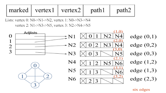
In contrast, adjacency multilists represent each edge only once, but both endpoints point to it using shared references (pointers).
Each edge is connected to two linked lists one for each vertex it connects.
Structure of an Adjacency Multilist Node
Each edge node in the multilist contains:
vertex1: one endpointvertex2: the other endpointnext1: link to the next edge invertex1's edge listnext2: link to the next edge invertex2's edge list- (optional)
weight: if the graph is weighted
Each vertex maintains a pointer to the head of its edge list.
Example
Let’s take a simple undirected graph.
A --- B
 \   /
   C
Vertices: A = 0, B = 1, C = 2 and Edges: (A–B), (A–C), (B–C)
Edge Nodes:
| Edge (u–v) | vertex1 | vertex2 | next1 (for u) | next2 (for v) |
|---|---|---|---|---|
| A–B | A | B | → A–C | → B–C |
| A–C | A | C | NULL | → B–C |
| B–C | B | C | NULL | NULL |
Each vertex points to its list of edges:
A→ A – B → A – CB→ A – B → B – CC→ A – C → B – C
Advantages of Adjacency Multilists
- Avoids duplication of edge information in undirected graphs.
- Can be more memory efficient than adjacency lists when storing large undirected graphs.
- Edge deletion is easier since you can directly remove a shared edge from both endpoints.
Disadvantages of Adjacency Multilists
- More complex to implement and maintain compared to adjacency lists.
- Not suitable for directed graphs.
- Not commonly supported in standard libraries or frameworks.
Applications of Adjacency Multilists
Efficient in applications where:
- Memory efficiency matters
- Frequent edge deletion or updates are needed
- Graph is undirected